What problem are we trying to solve?⌗

Have you ever wondered how does your favourite programming language’s standard library compute the values of $\sin(\theta)$, $\cos(\theta)$ and other trigonometric functions?

There are many ideas that might come to your mind. First, we might use the reflective property for negative arguments (e.g. $\sin(-\theta)=-\sin(\theta)$ holds), to bring the argument into range $<0, \infty>$. Then, the full period shift could be used to further reduce the range to $<0, 2\pi>$, yielding the $\sin(\theta + 2k\pi) = \sin(\theta)$ for $k \in Z$ formula. While there are more interesting tricks to further reduce the domain for easier computations, we can’t repeat these steps forever.

Using just mathematical insight, we’ve established that computing $\sin(\theta)$ for $\theta \in <-\pi, \pi>$ is enough to tell the values of $\sin(\theta)$ for all $\theta \in R$. There are many possibilities to follow from there, for example, using the ridiculous (but valued by engineers) approximation $\sin(\theta) = \theta$ combined with some more properties:

Although, such an approximation is generally too inaccurate for many use cases, so a different method has to be used. Currently, the values of $\sin(\theta)$ are nuemrically approximated using two mathematical devices - the Chebyshev polynomials and the Taylor series.

Since it’s not the first time Chebyshev polynomials are a little star of my blog post, today I’d like to demonstrate my implementation of the Taylor series in APL.

What is Taylor Series anyway?⌗

Assuming that the $n$-th derivative at point $a$ of $f(x)$ computable, it is possible to express the function as an infinite sum of terms using the Taylor Series. Since infinite sums are generally not useful to numerical methods, we (almost) always use a partial sum formed by the first few terms of a Taylor series. Taylor polynomials (for a given $n$, where $n + 1$ terms of a Taylor series is a polynomial of degree $n$) are approximations of a function, which become generally better as $n$ increases.

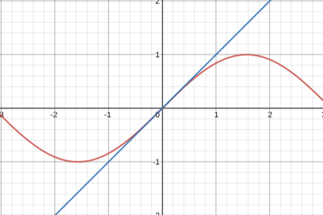
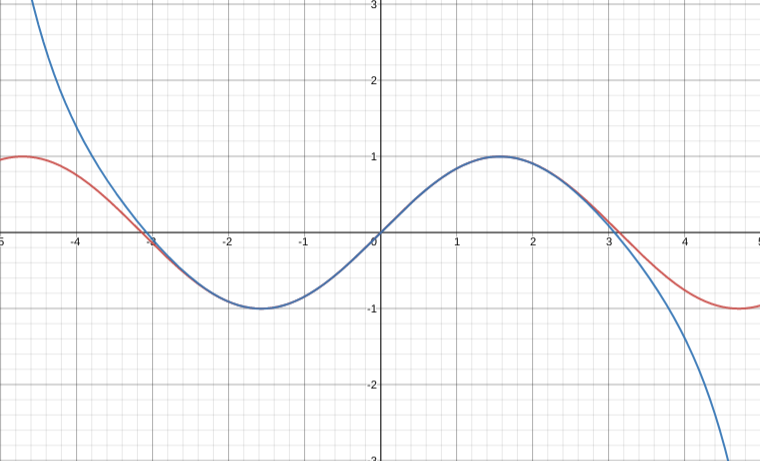
A famours approximation of $\sin(x)$ derived using Taylor Series is demonstrated below.

$$\sin(x) \approx x - \frac{x^3}{3!} + \frac{x^5}{5!} - \frac{x^7}{7!}$$

Implementing Taylor Series.⌗

The general formula for Taylor series is fairly straightforward and it’s the basis for my implementation in APL:

$${\displaystyle f(a)+{\frac {f’(a)}{1!}}(x-a)+{\frac {f’’(a)}{2!}}(x-a)^{2}+{\frac {f’’’(a)}{3!}}(x-a)^{3}+\cdots ,}$$

The first immediate concern is computing the values of the $n$-th derivative of $f$. Recalling the definition of a derivative:

$$f’(a)=\lim _{h\to 0}{\frac {f(a+h)-f(a)}{h}}$$

I arbitrarily pick a small value of $h$ and thus approximate the derivative in point:

h←0.01 ⋄ D←{h÷⍨⍵-⍥⍺⍺⍨⍵+h}

It’s not the end of the story just yet, though, since it’s not just the first derivative what’s needed. An important (and somewhat trivial) observation is that one can apply the $D$ operator $n$ times to get the $n$-th derivative!

      {⍵*2}D 1
2.01
      {⍵*2}D D 1
2
      {⍵*2}D D D 1
0

Verifying the computations, $\frac{df}{dx}=2x$, $\frac{d^2f}{dx^2}=2$ and finally $\frac{d^3f}{dx^3}=0$, so the results seem to be correct. Unfortunately, there is no way to apply an operator given amount of times to a function (analogically to the existing ⍣ for functions), so I had to roll my own recursive $n$-th derivative function:

ND←{⍵⍵=1:⍺⍺ D ⍵ ⋄ ((⍺⍺ D) ∇∇ (⍵⍵-1)) ⍵}

In the end, it’s nothing too complicated - first derivative marks the end of recursion, the second derivative is the first derivative of the first derivative, and so on. Additionally, I decided to hardcode the degree of the Taylor polynomial that is going to be computed using n←4.

Assuming the ⍵ parameter to the taylor function is the point at which an existing taylor polynomial is evaluated, my implementation is almost ready:

taylor←{
    h←0.01 ⋄ n←4 ⋄ f←⍺⍺ ⋄ a←⍵⍵ ⋄ D←{h÷⍨⍵-⍥⍺⍺⍨⍵+h}
    ND←{⍵⍵=1:⍺⍺ D ⍵ ⋄ ((⍺⍺ D)∇∇(⍵⍵-1))⍵}
    +/⍵∘T¨⍳n
}

The final line will map a function that generates Taylor polynomial terms to build the final approximation at point. Recalling the expression above, the implementation will diverge into two branches:

T←{
    ⍵=0:f a
    ((f ND ⍵⊢a)÷!⍵)×⍵*⍨⍺-a
}

The 0-th term of the Taylor polynomial is always $f(a)$, while the next ones follow the standard formula:

$${\displaystyle {\frac {f^{(n)}(a)}{n!}}(x-a)^{n},}$$

where $f^{(n)}(a)$ is the $n$-th derivative of $f$ at point $a$.

Testing⌗

I test my implementation as follows:

range←3×((-∘⌽,⊢)⍳÷⊢)30
]plot range ({1○⍵}¨range) (({1○⍵}taylor 0)¨range)

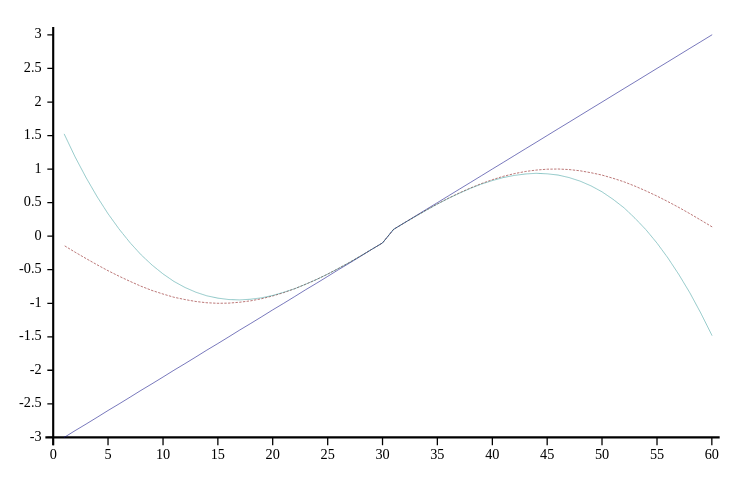
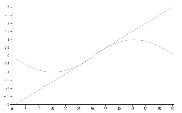
It appears that my implementation is fairly close to being acceptably accurate, but I can make it better by increasing the Taylor polynomial degree to n←7:

Summary⌗

I believe that this tiny Taylor Series implementation in APL is somewhat unique, since it conveys many concepts of mathematics in an almost verbatim way. There’s an incredibly obvious link to notice between the last line of my implementation:

+/⍵∘{((f ND ⍵⊢a)÷!⍵)×⍵*⍨⍺-a}¨⍳n

… and the actual mathematical formula:

$${\displaystyle \sum _{n=0}^{\infty }{\frac {f^{(n)}(a)}{n!}}(x-a)^{n},}$$

It’s a proof (or rather a demonstration) of sorts that APL is well-suited for representing concepts in mathematics that overlap with numerical methods and actual computation. Finally, the full source code follows:

taylor←{
    h←0.01 ⋄ n←4 ⋄ f←⍺⍺ ⋄ a←⍵⍵ ⋄ D←{h÷⍨⍵-⍥⍺⍺⍨⍵+h}
    ND←{⍵⍵=1:⍺⍺ D ⍵ ⋄ ((⍺⍺ D)∇∇(⍵⍵-1))⍵}
    +/⍵∘{
        ⍵=0:f a
        ((f ND ⍵⊢a)÷!⍵)×⍵*⍨⍺-a
    }¨⍳n
}