Triangulation of convex polygons

In this brief article, I will discuss the preliminaries of polygon triangulation using the APL programming language. Triangulation is an important concept in computational geometry, and it has applications in various fields, such as computer graphics, mesh generation, and finite element analysis. Triangular meshes are often used to represent surfaces in computer graphics, and they are also used in finite element analysis to approximate the solution of partial differential equations.

Introduction⌗

A convex polygon is a polygon in which all its interior angles are less than 180 degrees with vertices defined by $V = {(x_1, y_1), (x_2, y_2), \ldots, (x_n, y_n)}$, where $n$ is the number of vertices. Triangulation is the partitioning of a polygon with $n$ vertices into $n-2$ triangles by adding $n-3$ non-intersecting diagonals, which connect non-adjacent vertices.

Due to Euler, the total amount of ways to triangulate a $n$-gon is given by the $(n-2)$-th Catalan number:

$$C_n = \frac{1}{n+1}\binom{2n}{n}$$

Asymptotically, Catalan numbers grow as:

$$C_n \sim \frac{4^n}{n^{3/2}\sqrt{\pi}}$$

Consequently, the algorithm enumerating all possible triangulations of a polygon is exponential in time complexity.

Unconstrainted triangulation⌗

If we wish to triangulate a polygon without any constraints, the fan triangulation of any polynomial can be computed in linear time:

Once we pick a starting vertex $v_0$, we can connect it to all other vertices $v_1, v_2, \ldots, v_{n-1}$, creating $n-2$ triangles.

Another method of unconstrained triangulation is the ear-clipping algorithm, which is computed in $\mathcal O(n^2)$ time. The algorithm iteratively removes “ears” from the polygon, where an ear is a triangle with two consecutive edges of the polygon and the third edge inside the polygon. We begin the implementation with a function that given three points determines if they form a convex angle:

Sign←{a b c←⍵⋄(b-a)-.×⌽c-a}
Convex←0∘≤ Sign

The next step is to determine, given a point $p$, whether it lies inside the triangle $abc$. For this purpose, we could make use of barycentric coordinates, but the naive method (checking on which side of the half-plane created by the edges the point resides) is sufficient for our purposes:

InTriangle←{a b c←⍵⋄0 (~∨.<∧∨.>) Sign¨ (⍺ a b) (⍺ b c) (⍺ c a)}

The method for finding the ears is then straightforward. We return the ear and the rest of the polygon in a tuple. We implement checks in order to determine if the polygon is large enough, then iterate over the consecutive 3-triplets of vertices, to then determine if they form an ear. The first ear found is returned and its vertex is removed from the polygon.

Ear←{
  3>≢⍵:⍬ ⍬⋄3=≢⍵:⍵ ⍬
  V←3,/(2+≢⍵)⍴¯1⌽⊂¨⍵
  S←⍵∘{
    ~Convex ⍵:1
    ∨/(InTriangle∘⍵∧~∘(∊∘⍵)∘⊂)¨⍺}¨V
  E←V⊃⍨S⍳0⋄E(⍵~⊂2⊃E)}

The triangulation function successively removes ears from the polygon until only three vertices remain and returns the resulting triangulation:

Triangulate←{⍺←⍬⋄3>≢⍵:⍺⋄e r←Ear⍵⋄(⍺,⊂e)∇r}

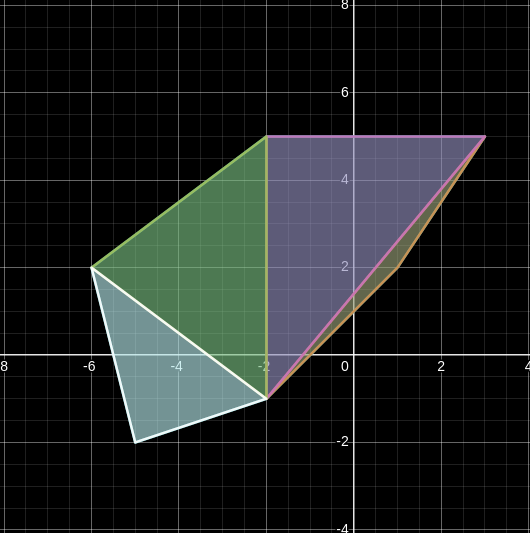
To test our code, we will use the following polygon:

polygon←(1 2) (3 5) (¯2 5) (¯6 2) (¯5 ¯2) (¯2 ¯1)

We will also plot it using Desmos:

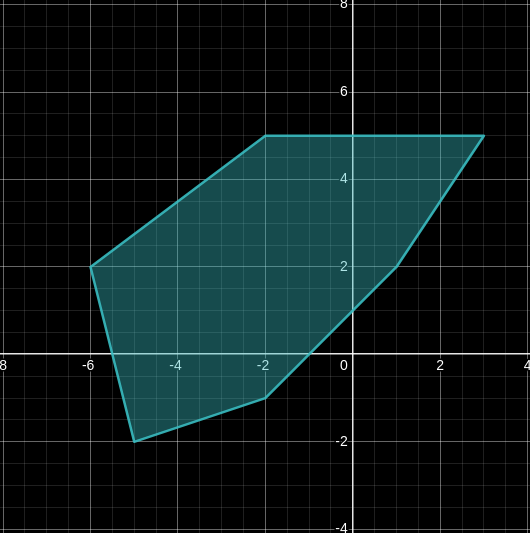
The resulting triangulation is given by:

  Triangulate polygon
┌───────────────┬────────────────┬─────────────────┬──────────────────┐
│┌─────┬───┬───┐│┌─────┬───┬────┐│┌─────┬────┬────┐│┌────┬─────┬─────┐│
││¯2 ¯1│1 2│3 5│││¯2 ¯1│3 5│¯2 5│││¯2 ¯1│¯2 5│¯6 2│││¯6 2│¯5 ¯2│¯2 ¯1││
│└─────┴───┴───┘│└─────┴───┴────┘│└─────┴────┴────┘│└────┴─────┴─────┘│
└───────────────┴────────────────┴─────────────────┴──────────────────┘

Constrained triangulation⌗

Suppose that we wish to triangulate a $n$-gon into $n-2$ triangles $T = {t_1, t_2, \ldots, t_{n-2}}$, where each triangle $t_i$ is defined by the vertices $v_i = {v_{i1}, v_{i2}, v_{i3}}$. We can then define a cost function $f : T \to \mathbb R$ that assigns a cost to each triangle. The cost function can be defined in various ways, such as the area of the triangle, the length of the edges, or the angle between the edges. The constrained triangulation problem is then to find the cost of the triangulation that minimizes the cost function.

Suppose that we have the following cost function, which assigns the cost of a triangle to be the sum of the lengths of its edges:

Cost←{1⊥(1⊥×⍨⍤-)/¨0 1 2(2∘↑⌽)¨⊂⍵}

The naive solution to this problem runs in exponential time through testing all possible triangulations:

MTC←{
  ⍺←1,≢⍵⋄i j←⍺⋄j<i+2:¯1
  ⌊/⍵∘{(i ⍵ MTC ⍺)+(⍵ j MTC ⍺)+Cost⍺[i j ⍵]}¨i+⍳j-i+1}

Nonetheless, for small polygons, it’s rather fast:

  MTC polygon
261
  'cmpx'⎕cy'dfns'
  cmpx 'MTC polygon'
2.9E¯4

We can improve upon this solution making use of Dynamic Programming: Many recursive calls in the naive solution are repeated, so we can store the results of these calls in a table and use them to avoid recomputation. We accomplish it via the use of the memo operator from the dfns workspace:

dpMTC←{
  P←⍵⋄f←{
    i j←⍵⋄j<i+2:¯1
    ⌊/{(f i ⍵)+(f ⍵ j)+Cost P[i j ⍵]}¨i+⍳j-i+1
  }memo(cache'')
  f 1,≢P}