Finding the roots of a polynomial can be very helpful if one aims to factorise it. Sometimes, solving a polynomial equation $W(x) = 0$ can yield useful mathematical quantities. For instance, finding the roots of the characteristic polynomial of a matrix will yield its eigenvalues.

The Newton-Raphson and Secant method⌗

The Newton-Raphson method is probably the most popular approach to numerically approximating roots. I decided against using it for a few reasons. Since the function I’m working with is a blackbox function, I’d need to take the derivative in point of it. It’s something that I’ve covered in the past, but I can do something better (and more interesting!) this time. The Secant method is more practical and realistic for my use case. It can be thought of as a finite-difference approximation of Newton’s method, which in the end is all numerical methods are capable of.

$$\Delta f(x)=f(x+1)-f(x)$$

Unsurprisingly, the secant method just like the Newton’s method can be described as a recurrence relation:

$${\displaystyle x_{n}=x_{n-1}-f(x_{n-1}){\frac {x_{n-1}-x_{n-2}}{f(x_{n-1})-f(x_{n-2})}}}$$

Which follows from a finite difference approximation:

$${\displaystyle f’(x_{n-1})\approx {\frac {f(x_{n-1})-f(x_{n-2})}{x_{n-1}-x_{n-2}}}.}$$

To demonstrate the Secant method using APL, I will take a simple function and try to find one of its roots. Starting with $f(x) = x^2-5$, using the above formula verbatim, I arrived at the following operator:

secant←{
  f←⍺⍺⋄{
    ⍵≤1:⍵⋄g←⊃v←∇¨⍵-1 2
    g-(f g)×(⊢÷⍥(-/)f¨)v
  }⍵
}

The code assumes that $x_0 = 0$ and $x_1 = 1$. There isn’t much to unpack - the vector v is just $x_{n-1}$ and $x_{n-2}$, so consequently g is $x_{n-1}$. The train below is a bit confusing, but ⊢÷⍥(-/)f¨ is equivalent to (-/⊢)÷(-/f¨), which simply divides the difference $x_{n-1} - x_{n-2}$ and $f(x_{n-1}) - f(x_{n-2})$.

With 10 iterations of the algorithm, I arrive at the following:

  f←5-⍨×⍨
  f secant 10
2.236067977

… which appears to indeed be one of the roots. But that’s not what I’m really after!

The Weierstrass method⌗

The Weierstrass method can be used to numerically find the solutions to an equation $W(x) = 0$. There are a few good things about it, but the most important one is that it finds all the roots of the polynomial, no matter if they’re complex or real, and allows us to completely factorise the polynomial - simply speaking, turn it into a product of polynomials of first degree.

We can demonstrate the Weierstrass method on a simple polynomial:

$$W(x) = x^3 + ax^2 + bx + c$$

We can rewrite $W(x)$ as a product, as mentioned earlier.

$$W(x) = (x - x_0) (x - x_1) (x - x_2)$$

The next steps are very similar to the Newton’s method. For sufficiently big $n$, $p_n \approx x_0$, $q_n \approx x_1$ and $r_n \approx x_2$. We pick $p_0$, $q_0$ and $r_0$ as next powers (starting with the $0$-th power) of a complex number which is neither real nor a de Moivre number. The formulae follow:

$${\displaystyle p_{n}=p_{n-1}-{\frac {f(p_{n-1})}{(p_{n-1}-q_{n-1})(p_{n-1}-r_{n-1})}}}$$

$${\displaystyle q_{n}=q_{n-1}-{\frac {f(q_{n-1})}{(q_{n-1}-p_{n-1})(q_{n-1}-r_{n-1})}}}$$

$${\displaystyle r_{n}=r_{n-1}-{\frac {f(r_{n-1})}{(r_{n-1}-p_{n-1})(r_{n-1}-q_{n-1})}}}$$

While the usual Weierstrass method attempts to use $p_n$ in definitions of $q_n$ and $r_n$, my modified version of it decides against it to simplify the implementation at the cost of precision thus having to perform more iterations of the algorithm.

The implementation⌗

I start my implementation of the Weierstrass algorithm by creating a function that evaluates the polynomial at a point. Since the Weierstrass algorithm requires the largest power of $x$ to have the coefficient $1$, I adjust for that:

solve←{
  f←⊥∘((⊢÷⊃)⍵)
}

Since the algorithm will juggle around the values of $W(x)$ and $x$ in a table, I add a function that will build it from given values of $x$:

solve←{
  f←⊥∘((⊢÷⊃)⍵)⋄g←{⍵⍪⍉⍪f¨⍵}
}

Before the first iteration of the algorithm, I create a table of $p_0$, $q_0$, …, with the starting values equal to the next powers of 0.4J0.9.

solve←{
  f←⊥∘((⊢÷⊃)⍵)⋄g←{⍵⍪⍉⍪f¨⍵}
  g 0.4J0.9*⎕io-⍨⍳1-⍨≢⍵
}

Since the algorithm iteration will take the table as the input, I’m interested only in the first row ($x$ values), since the second row will always ideally be zero. Additionally, I’d like to round the results a little, preferably according to the comparison tolerance, so that very small real/imaginary values are truncated (since they’re most certainly insignificant). Additionally, the iteration function will be executed as many times as ⍺ which purposefully doesn’t have a default value:

solve←{
  f←⊥∘((⊢÷⊃)⍵)⋄g←{⍵⍪⍉⍪f¨⍵}
  {+/¯9 ¯11○(⊢×⎕ct<|)9 11○⍵}¨,1↑{
    ⍝ ...
  }⍣⍺ g 0.4J0.9*⎕io-⍨⍳1-⍨≢⍵
}

Now, for the most difficult part - the iteration function. I start by extracting the current values of zeroes:

solve←{
  f←⊥∘((⊢÷⊃)⍵)⋄g←{⍵⍪⍉⍪f¨⍵}
  {+/¯9 ¯11○(⊢×⎕ct<|)9 11○⍵}¨,1↑{
    v←,1↑⍵
  }⍣⍺ g 0.4J0.9*⎕io-⍨⍳1-⍨≢⍵
}

Then, I fold the matrix with the single iteration function and build a table out of it’s results:

solve←{
  f←⊥∘((⊢÷⊃)⍵)⋄g←{⍵⍪⍉⍪f¨⍵}
  {+/¯9 ¯11○(⊢×⎕ct<|)9 11○⍵}¨,1↑{
    v←,1↑⍵⋄g{ ... }⌿⍵
  }⍣⍺ g 0.4J0.9*⎕io-⍨⍳1-⍨≢⍵
}

The function is given the $x$ and $y$ values as ⍺ and ⍵:

solve←{
  f←⊥∘((⊢÷⊃)⍵)⋄g←{⍵⍪⍉⍪f¨⍵}
  {+/¯9 ¯11○(⊢×⎕ct<|)9 11○⍵}¨,1↑{
    v←,1↑⍵⋄g{⍺-⍵÷×/0~⍨⍺-v}⌿⍵
  }⍣⍺ g 0.4J0.9*⎕io-⍨⍳1-⍨≢⍵
}

The correspondence between the iteration function and the formula above is obvious. As a little trick, to avoid having to remove the current zero from the v matrix, I simply remove the zeroes from the result of subtraction. Then, the product of them divides the value of $W(x)$ and this all is subtracted from the current $x$ value.

That’s a lot to unpack, but let’s test the implementation now. As a small spoiler for my future blog post, where I’ll be explaining eigenvalues, determinants and inverse matrices using the Faddeev-LeVerrier algorithm, I will compute the characteristic polynomial of a simple matrix:

  data
3 1 5
3 3 1
4 6 4
  faddeev_leverrier data
1 ¯10 4 ¯40

Since eigenvalues are just the roots of the characteristic polynomial, I attempt finding them using my new toy:

  50 solve 1 ¯10 4 ¯40 
0J2 0J¯2 10

Let’s verify the eigenvalues I obtained using pencil and paper calculations. From the definition of the eigenvector $v$ corresponding to the eigenvalue $\lambda$:

$$A v = \lambda v$$

I also know that:

$$A v = \lambda v = (A - \lambda I) \cdot v = 0$$

Still, by definition, the equation has a nonzero solution if and only if:

$$\det(A - \lambda I) = 0$$

Next up, I get the following:

$$\det(A - \lambda I) = \begin{vmatrix} 3 - \lambda & 1 & 5\\ 3 & 3 - \lambda & 1\\ 4 & 6 & 4 - \lambda \end{vmatrix} = - \lambda^3 + 10\lambda^2 - 4\lambda + 40$$

… which is the characteristic polynomial obtained earlier. Continuing:

$$-\lambda^3 + 10\lambda^2 - 4\lambda + 40 = - (\lambda - 10) (\lambda^2 + 4) = 0$$

It is obvious that the first root is 10, while the other two are solutions to $x^2 + 4 = 0$. Using the standard method of obtaining roots of a quadratic polynomial, I conclude that the other two roots are (unsurprisingly) conjugates of each other and equal to $2i$ and $-2i$. Finding the eigenvectors (which is out of scope of the current post) is left as an exercise to the reader.

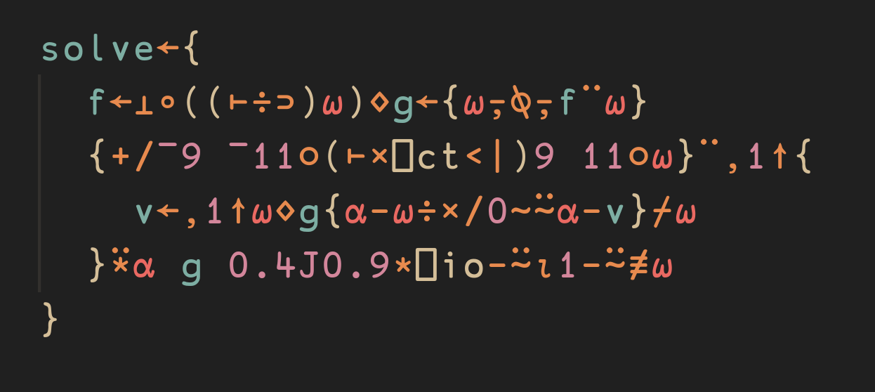
Summary⌗

The current, third post of my “in APL” series demonstrates how beautifully and naturally certain mathematical concepts can be expressed using APL. The full source code for this blog post follows:

secant←{
  f←⍺⍺⋄{
    ⍵≤1:⍵⋄g←⊃v←∇¨ ⍵-1 2
    g-(f g)×(⊢÷⍥(-/)f¨)v
  }⍵
}

solve←{
  f←⊥∘((⊢÷⊃)⍵)⋄g←{⍵⍪⍉⍪f¨⍵}
  {+/¯9 ¯11○(⊢×⎕ct<|)9 11○⍵}¨,1↑{
    v←,1↑⍵⋄g{⍺-⍵÷×/0~⍨⍺-v}⌿⍵
  }⍣⍺ g 0.4J0.9*⎕io-⍨⍳1-⍨≢⍵
}