Lempel-Ziv factorisation for file type detection.

Currently we have access to various tools to detect the type of data that we are dealing with. Ranging from file to the fancy and new magika from Google or binwalk. However, sometimes such sophisticated tools either provide us with too much or too little information from the perspective of a data compressor.

The purpose of segmentation and file type detection is clear: if we know the precise data type that we are dealing with (e.g. BMP graphics, WAV audio, etc.), we can apply a more efficient algorithm for this data type compared to a weaker but more general fallback method. Further, segmentation improves the compression ratio by allowing us to discard irrelevant context more efficiently; while this is not particularly helpful to Lempel-Ziv codecs, statistical codecs and especially Burrows-Wheeler transform-oriented codecs improve in compression ratio. For example, the following table illustrates the compression ratio of various compression codecs on the Calgary Corpus, a collection of files that are commonly used to benchmark compression algorithms:

With the Calgary corpus, we have it easy: the files are trivially segmented (just extract the zip file!) and we can easily detect the file type just by looking at the file extension. Dealing with real world data is unfortunately not so simple, so it is necessary to develop some sort of heuristic to chop a file into segments.

Prior art⌗

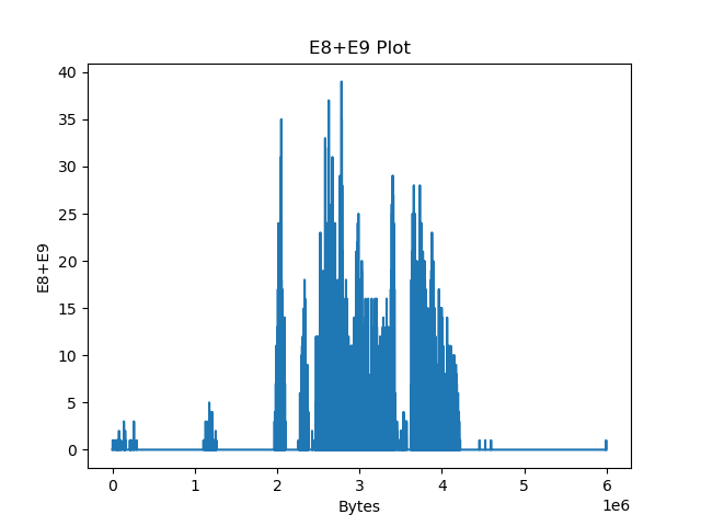
Existing compressors such as bsc or variations of paq8 can already segment and detect file types (latter: only paq8l). In this blog post we will be primarily focusing on detecting executable content. paq8l (which employs a more sophisticated technique for this) simply counts the occurences of particular byte values (E8 and E9 - opcodes of the jmp and call instructions) in a window to tag the data as executable:

Filetype detect(FILE* in, int n, Filetype type) {
  U32 buf1=0, buf0=0;  // last 8 bytes
  long start=ftell(in);

  // For EXE detection
  Array<int> abspos(256),  // CALL/JMP abs. addr. low byte -> last offset
    relpos(256);    // CALL/JMP relative addr. low byte -> last offset
  int e8e9count=0;  // number of consecutive CALL/JMPs
  int e8e9pos=0;    // offset of first CALL or JMP instruction
  int e8e9last=0;   // offset of most recent CALL or JMP

  for (int i=0; i<n; ++i) {
    int c=getc(in);
    if (c==EOF) return (Filetype)(-1);
    buf1=buf1<<8|buf0>>24;
    buf0=buf0<<8|c;

    // Detect EXE if the low order byte (little-endian) XX is more
    // recently seen (and within 4K) if a relative to absolute address
    // conversion is done in the context CALL/JMP (E8/E9) XX xx xx 00/FF
    // 4 times in a row.  Detect end of EXE at the last
    // place this happens when it does not happen for 64KB.

    if ((buf1&0xfe)==0xe8 && (buf0+1&0xfe)==0) {
      int r=buf0>>24;  // relative address low 8 bits
      int a=(buf0>>24)+i&0xff;  // absolute address low 8 bits
      int rdist=i-relpos[r];
      int adist=i-abspos[a];
      if (adist<rdist && adist<0x1000 && abspos[a]>5) {
        e8e9last=i;
        ++e8e9count;
        if (e8e9pos==0 || e8e9pos>abspos[a]) e8e9pos=abspos[a];
      }
      else e8e9count=0;
      if (type!=EXE && e8e9count>=4 && e8e9pos>5)
        return fseek(in, start+e8e9pos-5, SEEK_SET), EXE;
      abspos[a]=i;
      relpos[r]=i;
    }
    if (type==EXE && i-e8e9last>0x1000)
      return fseek(in, start+e8e9last, SEEK_SET), DEFAULT;
  }
  return type;
}

However, we wish to do even better. We could settle on parsing the ELF/PE header to determine the precise locations of code and data, but this solution does not really generalise to other file types. Instead, we will assume that the data was already processed by a program that can detect and parse assets embedded in the executable at its own leisure (e.g. find BMP/gzip/WAV file headers), and focus on telling apart code segments and data segments.

Lempel-Ziv factorisation⌗

LZ factorisation is simply the process of finding the longest preceding match of the current search window and the current position. There are many techniques for this: linear scan, hash chains, Rabin-Karp, suffix trees - the list goes on. We will not be discussing these techniques in detail and assume that we already have a black-box device that can perform LZ factorisation, i.e. emit a sequence of MAT <len> <dist> and LIT <len> commands.

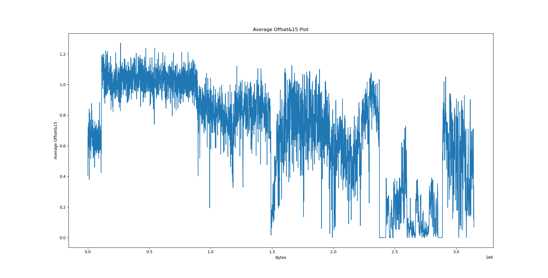
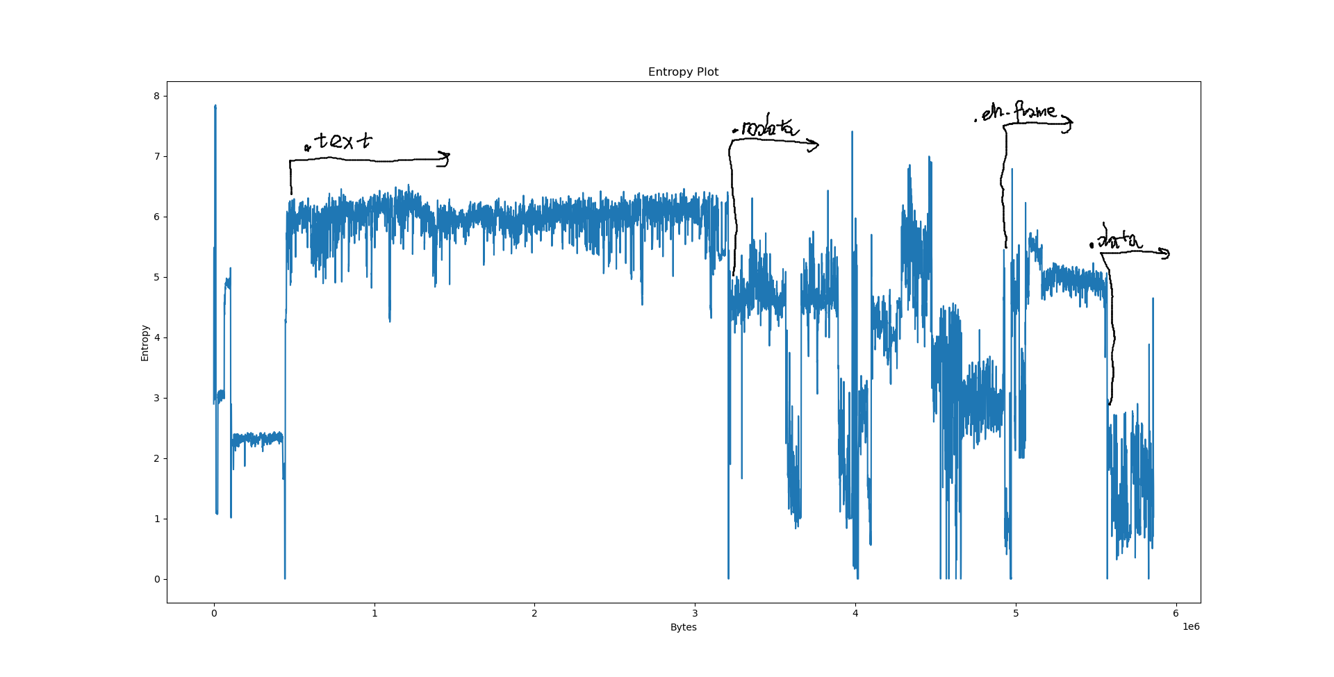
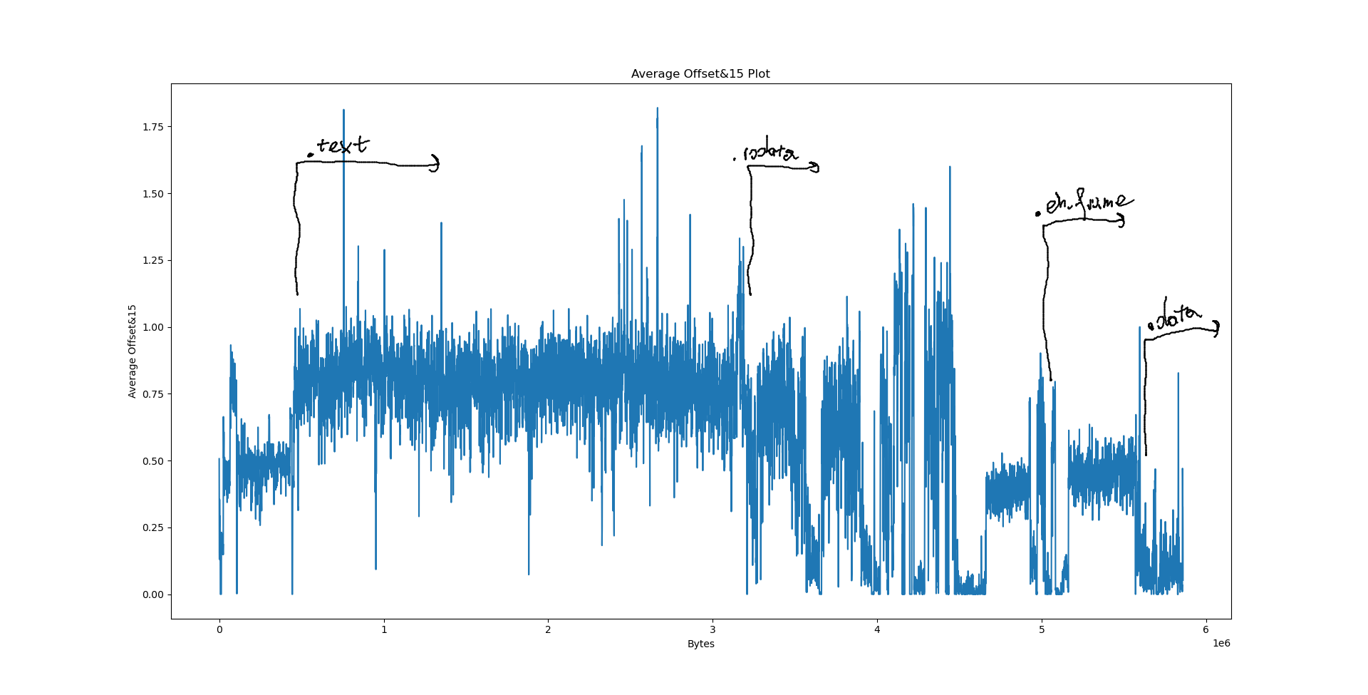
For this purpose, we will write a simple program that reads a file and its LZ factorisation to display a sliding window entropy plot and the sliding window average LZ factorisation offset masked to low order bits.

import sys
import os
import math
import matplotlib.pyplot as plt
from collections import defaultdict

def entropy(data):
    entropy = 0
    for x in range(256):
        p_x = float(data.count(x))/len(data)
        if p_x > 0:
            entropy += - p_x * math.log(p_x, 2)
    return entropy

def main():
    if len(sys.argv) != 3:
        print("Usage: python entropy-plot.py <filename> <LZ dump>")
        sys.exit(1)
    data = open(sys.argv[1], 'rb').read()
    lz_data = open(sys.argv[2], 'rb').read()
    entropies = []
    for i in range(0, len(data), 512):
        entropies.append(entropy(data[i:i+1024]))
    plt.plot(range(0, len(data), 512), entropies)
    plt.xlabel('Bytes')
    plt.ylabel('Entropy')
    plt.title('Entropy Plot')
    plt.show()
    pos = 0
    offsets = defaultdict(int) # Default value is 0
    for line in lz_data.splitlines():
        if line.startswith(b'MAT'):
            length, offset = line.split()[1:]
            offsets[pos] = int(offset) & 15
            pos += int(length) + 4
        elif line.startswith(b'LIT'):
            length = line.split()[1]
            pos += int(length)
    avg_offsets = []
    for i in range(0, len(data), 512):
        avg_offsets.append(sum(offsets.get(j, 0) for j in range(i, i+1024)) / 1024)
    plt.plot(range(0, len(data), 512), avg_offsets)
    plt.xlabel('Bytes')
    plt.ylabel('Average Offset&15')
    plt.title('Average Offset&15 Plot')
    plt.show()

if __name__ == '__main__':
    main()

Results⌗

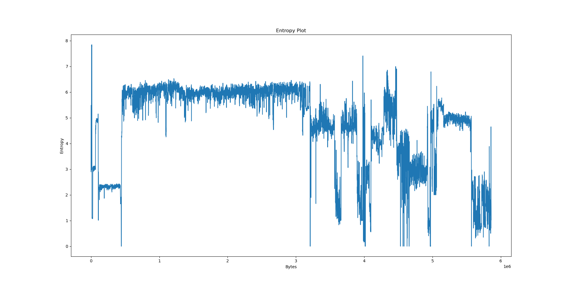
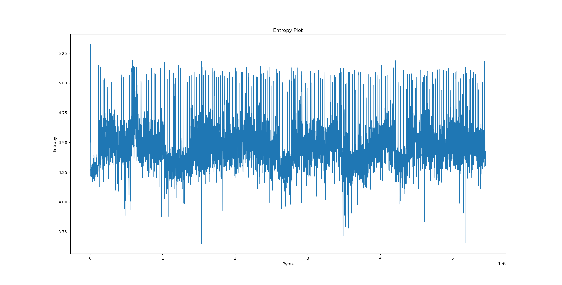
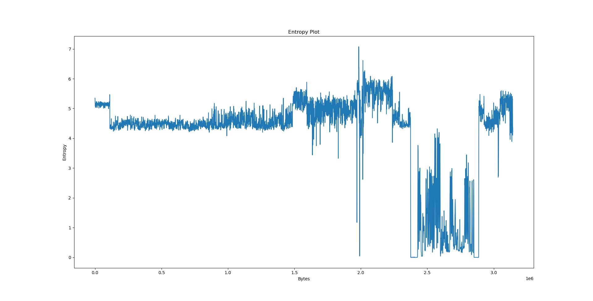
We will now consider three files: python3.10 coming from the Debian x86_64 package, data.txt - collected works of Shakespeare from Project Gutenberg and calgary.zip - the Calgary corpus. The results follow.

Interpreting the results⌗

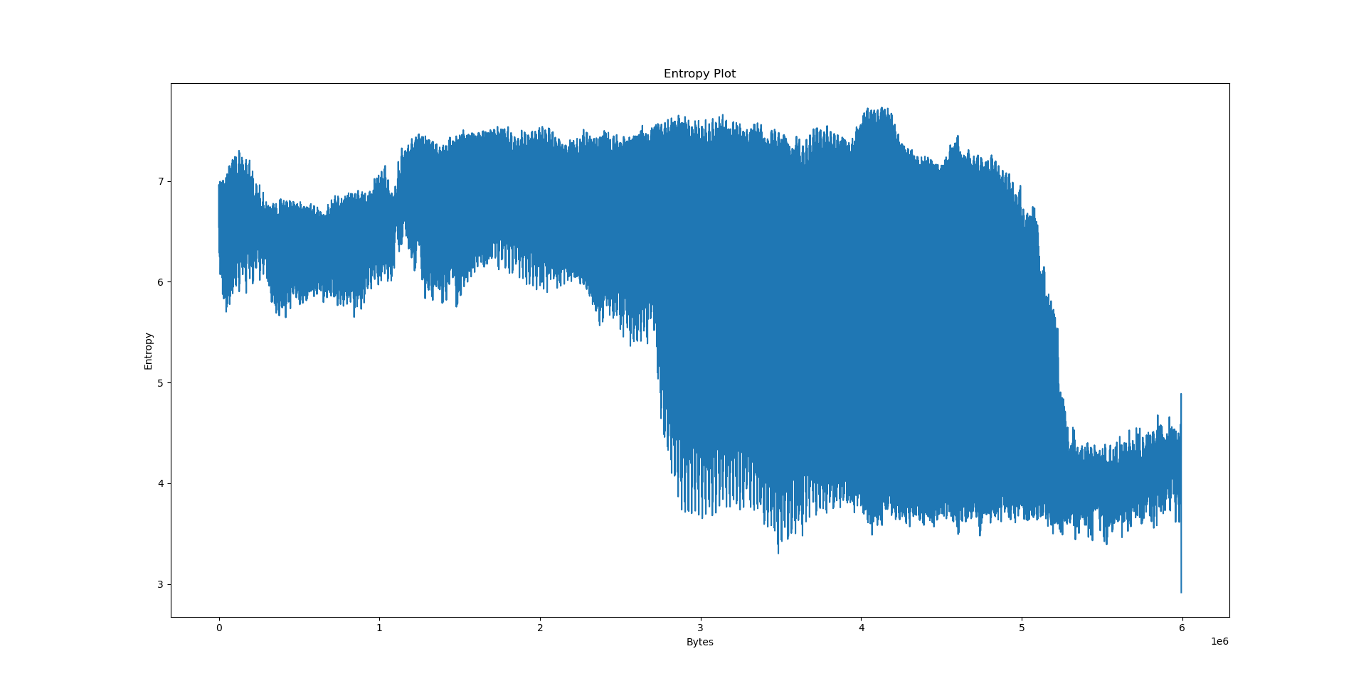
It’s the easiest to explain the results we have obtained on data.txt. By virtue of being text, its entropy is largely stationary. The offset plot is also not very meaningful and very uniform, since Lempel-Ziv models distances between occurences, and there is no particular pattern in the text that would cause the offset to be biased in any way - we would need a PPM model (or something even better) to detect such patterns.

We could speculate a lot about what the python3.10 graph actually wants to say, but we will consult readelf first.

Section Headers:
  [Nr] Name              Type            Address          Off    Size   ES Flg Lk Inf Al
  [ 0]                   NULL            0000000000000000 000000 000000 00      0   0  0
  [ 1] .interp           PROGBITS        0000000000000318 000318 00001c 00   A  0   0  1
  [ 2] .note.gnu.property NOTE            0000000000000338 000338 000020 00   A  0   0  8
  [ 3] .note.gnu.build-id NOTE            0000000000000358 000358 000024 00   A  0   0  4
  [ 4] .note.ABI-tag     NOTE            000000000000037c 00037c 000020 00   A  0   0  4
  [ 5] .gnu.hash         GNU_HASH        00000000000003a0 0003a0 003248 00   A  6   0  8
  [ 6] .dynsym           DYNSYM          00000000000035e8 0035e8 00cca8 18   A  7   1  8
  [ 7] .dynstr           STRTAB          0000000000010290 010290 0099a3 00   A  0   0  1
  [ 8] .gnu.version      VERSYM          0000000000019c34 019c34 00110e 02   A  6   0  2
  [ 9] .gnu.version_r    VERNEED         000000000001ad48 01ad48 0001b0 00   A  7   3  8
  [10] .rela.dyn         RELA            000000000001aef8 01aef8 04e750 18   A  6   0  8
  [11] .rela.plt         RELA            0000000000069648 069648 002a90 18  AI  6  26  8
  [12] .init             PROGBITS        000000000006d000 06d000 000017 00  AX  0   0  4
  [13] .plt              PROGBITS        000000000006d020 06d020 001c70 10  AX  0   0 16
  [14] .plt.got          PROGBITS        000000000006ec90 06ec90 0000b8 08  AX  0   0  8
  [15] .text             PROGBITS        000000000006ed50 06ed50 2a067e 00  AX  0   0 16
  [16] .fini             PROGBITS        000000000030f3d0 30f3d0 000009 00  AX  0   0  4
  [17] .rodata           PROGBITS        0000000000310000 310000 1c92c0 00   A  0   0 32
  [18] .stapsdt.base     PROGBITS        00000000004d92c0 4d92c0 000001 00   A  0   0  1
  [19] .eh_frame_hdr     PROGBITS        00000000004d92c4 4d92c4 013624 00   A  0   0  4
  [20] .eh_frame         PROGBITS        00000000004ec8e8 4ec8e8 063598 00   A  0   0  8
  [21] .init_array       INIT_ARRAY      00000000005505f0 5505f0 000008 08  WA  0   0  8
  [22] .fini_array       FINI_ARRAY      00000000005505f8 5505f8 000008 08  WA  0   0  8
  [23] .data.rel.ro      PROGBITS        0000000000550600 550600 005448 00  WA  0   0 32
  [24] .dynamic          DYNAMIC         0000000000555a48 555a48 000210 10  WA  7   0  8
  [25] .got              PROGBITS        0000000000555c58 555c58 000390 08  WA  0   0  8
  [26] .got.plt          PROGBITS        0000000000555fe8 555fe8 000e48 08  WA  0   0  8
  [27] .data             PROGBITS        0000000000556e40 556e40 03eb10 00  WA  0   0 32
  [28] .PyRuntime        PROGBITS        0000000000595960 595960 0002a0 00  WA  0   0 32
  [29] .probes           PROGBITS        0000000000595c00 595c00 000018 00  WA  0   0  2
  [30] .bss              NOBITS          0000000000595c20 595c18 0460b8 00  WA  0   0 32
  [31] .note.stapsdt     NOTE            0000000000000000 595c18 000290 00      0   0  4
  [32] .gnu_debuglink    PROGBITS        0000000000000000 595ea8 000034 00      0   0  4
  [33] .shstrtab         STRTAB          0000000000000000 595edc 00014c 00      0   0  1

Notably, we have a few big sections here: .data at 556e40, .eh_frame at 4ec8e8, .rodata at 310000 and .text at 06ed50. What happens if we try to pinpoint them on the plots?

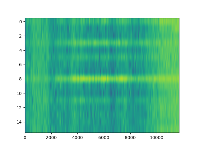
However, when it comes to LZ factorisation, averaging the match offsets doesn’t really win us that much. We can do better by looking at a proper heatmap of the match offsets and the distribution of E8/E9 bytes:

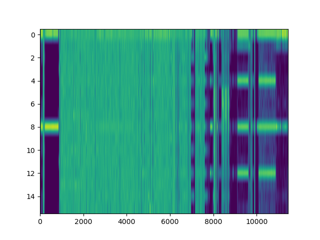
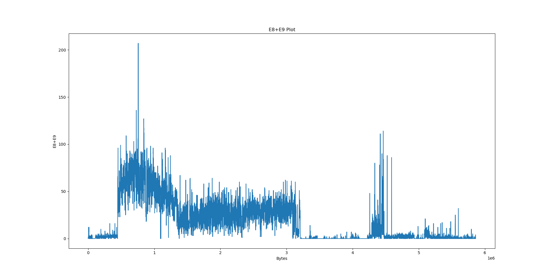
The machine code section is unfortunately not very well visible on the heatmap: After all, x86 opcodes are variable length. However, the E8/E9 plot is very clear: the machine code section is very well visible as a spike in the E8/E9 count. We can distinguish between random data (no LZ matches), text (no E8/E9 matches) and structured, non-machine-code data (e.g. BMP files, rigid structure of LZ matches, E8/E9 matches). What happens if we feed this program a WAV and BMP file?

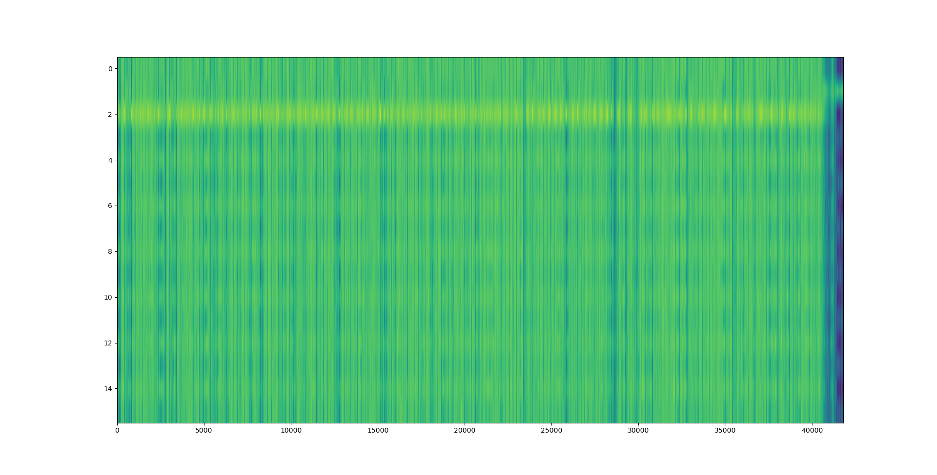
The bitmap file is a photo taken indoors by my phone’s camera.

As expected, the file has a more rigid structure, which lets us easily distinguish it from the other files. The same holds for the 16-bit WAV file, which has a lot of hits aligned at two bytes:

Takeaways⌗

Compression is an AI problem. Classification is an AI problem. Hence compression can be used for classification. There are many ways to apply compression algorithms in order to classify data (cf. as-of-recent famous gzip distance) and we have only scratched the surface. The compression models (results after delta encoding, entropy values, Lempel-Ziv match offsets, etc) can be used as input to neural networks that can learn to classify data more efficiently than existing approaches.